Instance Segmentation
Instance segmentation determines a pixel-wise mask for each object in an image. This tutorial explains how to generate source code for instance segmentation tasks using the cvtk package, train a model to perform instance segmentation, and run inference with the trained model. The overall workflow and even the generated source code are very similar to that of object detection.
Note
The cvtk package internally uses functions from torch (PyTorch), mmcv (MMCV), mmengine (MMEngine), and mmdet (MMDetection) packages for instance segmentation tasks. Make sure that torch, mmcv, mmengine, and mmdet are installed correctly without any errors before using cvtk.
import torch
import mmcv
import mmengine
import mmdet
print(f"torch {torch.__version__}")
print(f"mmcv {mmcv.__version__}")
print(f"mmengine {mmengine.__version__}")
print(f"mmdet {mmdet.__version__}")
Preparation
The cvtk deploy-model command can automatically generate Python source code for instance segmentation.
cvtk deploy-model --script_name segm.py --backend mmdet --task segm
This command generates a file named segm.py,
which contains simple source code for instance segmentation.
All complex functionality is imported from the cvtk package,
making the script easier to read and helping beginners understand the deep learning workflow.
By default, the Mask RCNN model (mask-rcnn_r101_fpn_1x_coco) is used.
Users can replace this with any other supported model by editing the generated script.
Available network architectures can be found in the MMDetection GitHub repository
(e.g., mmdetection.configs)
or by running the mim search command (e.g., mim search mmdet --model "mask-rcnn").
For users already familiar with deep learning,
it is recommended to run cvtk deploy-model with the --vanilla argument.
cvtk deploy-model --script_name segm.py --backend mmdet --task segm --vanilla
This generates a script that uses only torch and mmdet functions without relying on cvtk. Such a script can be shared with users who do not have cvtk installed or further customized, for example, by adding data augmentation or modifying the training loop.
Note
The source code generated for instance segmentation is almost the same as that for object detection, since both are based on the mmdet framework. The key differences are:
Network architecture: instance segmentation uses Mask RCNN (
mask-rcnn_r101_fpn_1x_coco), while object detection uses Faster RCNN (faster-rcnn_r101_fpn_1x_coco).Annotations: instance segmentation requires segmentation masks (pixel-level polygons), while object detection only requires bounding box coordinates.
Model Training and Validation
Training and validation can be performed by executing the generated source code, providing the training, validation, and test datasets along with the label file as follows. Note that the datasets must be in COCO format with segmentation mask coordinates.
python segm.py train \
    --label ./data/strawberry/label.txt \
    --train ./data/strawberry/train/segm.json \
    --valid ./data/strawberry/valid/segm.json \
    --test ./data/strawberry/test/segm.json \
    --output_weights ./outputs/strawberry.pth
The trained model weights will be saved in strawberry.pth.
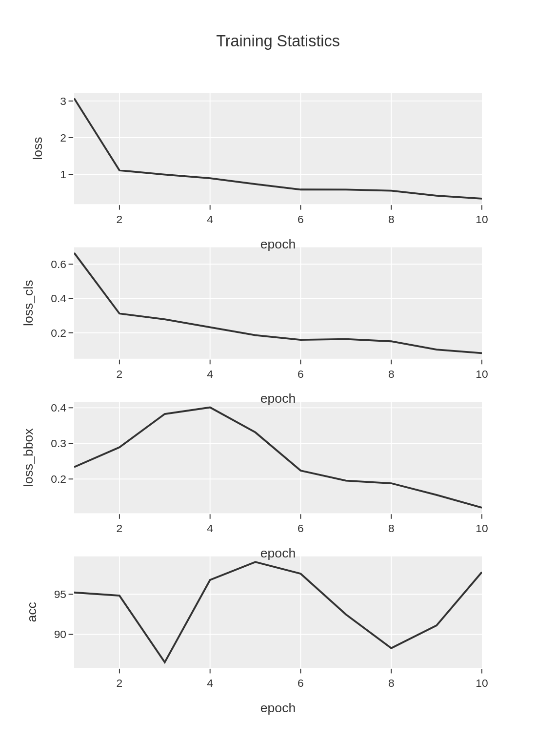
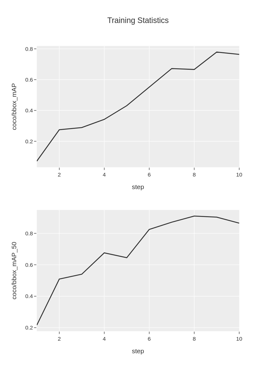
During training, loss and accuracy logs will be stored in
strawberry.train_stats.train.txt and strawberry.train_stats.valid.txt,
along with visualization figures generated from these files.
Both text files are tab-separated, for example:
strawberry.train_stats.train.txt
epoch       lr      data_time       loss    loss_rpn_cls    loss_rpn_bbox   loss_cls        acc     loss_bbox       loss_mask       time    memory
1   0.00118 0.03453 1.84487 0.03162 0.01490 0.59783 88.37890625     0.3763710225621859      0.8241304568946362      0.4096731980641683      5721.0
2   0.00238 0.01690 1.01754 0.01787 0.01174 0.31824 83.984375       0.4193130740523338      0.250374620705843       0.36697773933410643     5686.0
3   0.00353 0.01563 0.72365 0.00546 0.01157 0.21473 87.59765625     0.3275810395181179      0.1643025816977024      0.35318960666656496     5757.0
4   0.00478 0.01308 0.51533 0.00525 0.01162 0.15927 98.33984375     0.194721964225173       0.14444936953485013     0.37441123962402345     5804.0
5   0.00598 0.01276 0.44866 0.00665 0.01034 0.12237 95.3125 0.17035995483398436     0.13892668940126895     0.36310056209564207     5728.0
strawberry.train_stats.train.png
strawberry.train_stats.valid.txt
coco/bbox_mAP       coco/bbox_mAP_50        coco/bbox_mAP_75        coco/bbox_mAP_s coco/bbox_mAP_m coco/bbox_mAP_l coco/segm_mAP   coco/segm_mAP_50        coco/segm_mAP_75        coco/segm_mAP_s coco/segm_mAP_m coco/segm_mAP_l data_time       time    step
0.345       0.507   0.399   -1.0    -1.0    0.345   0.412   0.507   0.466   -1.0    -1.0    0.413   0.1388627529144287      0.86514892578125        1
0.352       0.614   0.345   -1.0    -1.0    0.352   0.5     0.614   0.581   -1.0    -1.0    0.501   0.012227217356363932    0.40663444995880127     2
0.579       0.748   0.693   -1.0    -1.0    0.582   0.643   0.748   0.748   -1.0    -1.0    0.659   0.01785115400950114     0.23407896359761557     3
0.642       0.785   0.785   -1.0    -1.0    0.642   0.72    0.785   0.785   -1.0    -1.0    0.75    0.018213987350463867    0.2121752897898356      4
0.643       0.829   0.829   -1.0    -1.0    0.643   0.718   0.829   0.829   -1.0    -1.0    0.725   0.01665182908376058     0.18859827518463135     5
strawberry.train_stats.valid.png
If test data is provided, the model will also be evaluated on it.
The inference results will be stored in the workspace (strawberry directory)
as test_outputs.coco.json in COCO format.
The test performance metrics (e.g., mAP) will be saved in strawberry.test_stats.json in JSON format.
The stats element summarizes mean metrics across all classes,
while per-class results are stored under class_stats:
{
    "stats": {
        "AP@[0.50:0.95|all|100]": 0.8671538582429673,
        "AP@[0.50|all|1000]": 0.9365079365079365,
        "AP@[0.75|all|1000]": 0.9365079365079365,
        ...
        "AP@[0.50:0.95|large|1000]": 0.8671538582429673,
        "AR@[0.50:0.95|all|100]": 0.4738095238095238,
        "AR@[0.50:0.95|all|300]": 0.9029761904761905,
    },
    "class_stats": {
        "flower": {
            "AP@[0.50:0.95|all|100]": 0.9252475247524753,
            "AP@[0.50|all|1000]": 1.0,
            "AP@[0.75|all|1000]": 1.0,
            ...
        },
        "green_fruit": {
            "AP@[0.50:0.95|all|100]": 0.9665016501650165,
            "AP@[0.50|all|1000]": 1.0,
            "AP@[0.75|all|1000]": 1.0,
            ...
        },
        "red_fruit": {
            "AP@[0.50:0.95|all|100]": 0.7097123998114098,
            "AP@[0.50|all|1000]": 0.8095238095238095,
            "AP@[0.75|all|1000]": 0.8095238095238095,
            ...
        }
    }
}
Inference
Performing inference using the trained model can be done directly from the command line.
The target images should be specified with the --data argument,
which can be either a text file containing image paths (one path per line)
or a directory containing images.
python segm.py inference \
    --label ./data/strawberry/label.txt \
    --data ./data/strawberry/test/images \
    --model_weights ./outputs/strawberry.pth \
    --output ./outputs/inference_results
The inference results for each image (i.e., images with predicted segmentation masks)
will be saved in the inference_results directory.
Additionally, a COCO format file containing all predicted annotations,
including bounding boxes and segmentation masks,
will be saved as instances.coco.json.
The following are examples of the output images.

