Object Detection

Object detection combines classification and localization to locate objects in an image through bounding boxes. This tutorial describes how to use the cvtk package to build a model of an object detection task, from training the to inference.

Note

The cvtk package internally calls functions implemented in the torch (PyTorch), mmcv (MMCV), and mmdet (MMDetection) packages for object detection tasks. Ensure that torch, mmdet, and mmcv is installed correctly without any errors before using the cvtk package.

import torch
import mmcv
import mmdet
print(torch.__version__)
print(mmcv.__version__)
print(mmdet.__version__)

Source Code Preparation

To generate Python source code, use the cvtk create command. For those new to programming or deep learning, it is recommended to run the following command to generate simple source code. The code generated by this command contains only the essential processes, with all complex processes imported from the cvtk package. This makes the source code easy to read and helps in understanding the flow of deep learning for beginners.

cvtk create --script det.py --task det

By default, Faster RCNN (faster-rcnn_r101_fpn_1x_coco) is used. Users can change the 'faster-rcnn_r101_fpn_1x_coco' part to any other network architecture by replacing it with another string in the generated source code. Available network architectures can be found on the MMDet GitHub repository (e.g., mmdetection.configs) or search by using the mim search command (e.g., mim search mmdet --model "r-cnn").

For those who are already familiar with deep learning, it is recommended to run the following command (cvtk create with the argument --vanilla) to generate source code that uses only the MMDetection package functions. Users can then customize the source code generated by this command to suit their needs. For example, users can add various processes such as data augmentation, optimization algorithms, and loss functions.

cvtk create --script det.py --task det --vanilla

Model Training and Validation

To train the model, open the source code generated above and execute it by providing training, validation, and test data to the input of the train function.

Alternatively, the source code can be executed directly from the command line as follows:

python det.py train \
    --label ./data/strawberry/label.txt \
    --train ./data/strawberry/train/bbox.json \
    --valid ./data/strawberry/valid/bbox.json \
    --test ./data/strawberry/test/bbox.json \
    --output_weights ./outputs/strawberry.pth

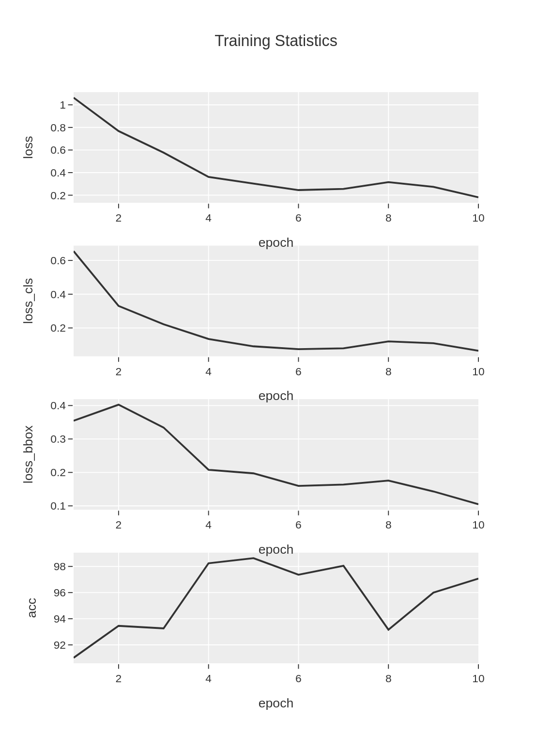
The weights of the trained model will be saved in strawberry.pth, and the loss and accuracy data during the training process will be saved in strawberry.train_stats.train.txt and strawberry.train_stats.valid.txt and the figures based on the two file. Both files are tab-separated files as follows:

strawberry.train_stats.train.txt

epoch       lr      data_time       loss    loss_rpn_cls    loss_rpn_bbox   loss_cls        acc     loss_bbox       time    memory
1   0.0011811623246492983   0.012568799654642741    1.0270314663648605      0.030940301870577967    0.019437399141800902    0.64003709902366        87.109375       0.3366166626413663      0.294748592376709       5539.0
2   0.0023823647294589174   0.002985730171203613    0.7621045112609863      0.018117828631657177    0.014595211343839764    0.33093497216701506     86.328125       0.39845649629831315     0.2621237087249756      5539.0
3   0.003583567134268537    0.0030106496810913086   0.5718079897761345      0.007945213937782683    0.012842701384797692    0.2135572835057974      90.8203125      0.33746279165148735     0.25948814868927        5540.0
4   0.004784769539078155    0.002938108444213867    0.3803089389204979      0.004043563161249039    0.012852981882169844    0.13384666815400123     98.828125       0.22956572577357293     0.25895278453826903     5539.0
5   0.005985971943887774    0.003097343444824219    0.3158286053687334      0.0028303257742663844   0.012002748951781541    0.10025690719485283     98.33984375     0.20073862358927727     0.2683125925064087      5540.0

strawberry.train_stats.train.png

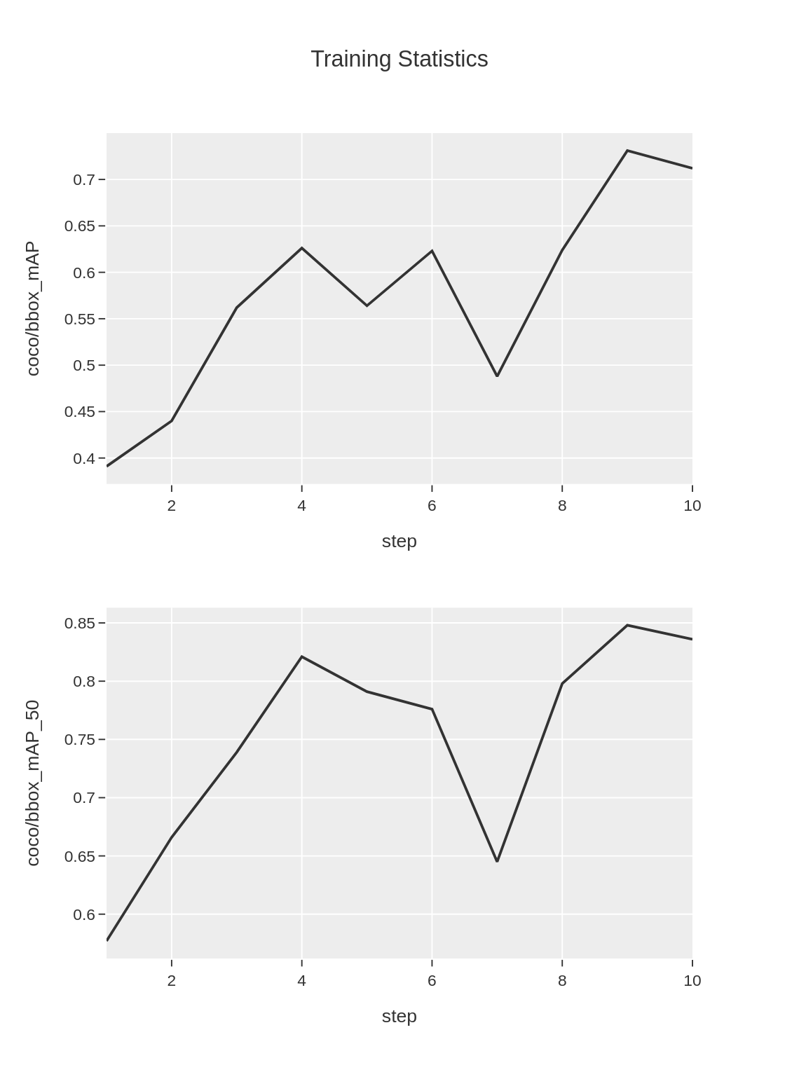
strawberry.train_stats.valid.txt

coco/bbox_mAP       coco/bbox_mAP_50        coco/bbox_mAP_75        coco/bbox_mAP_s coco/bbox_mAP_m coco/bbox_mAP_l data_time       time    step
0.324       0.444   0.37    0.0     -1.0    0.345   0.07410950660705566     0.1943049907684326      1
0.36        0.572   0.377   0.0     -1.0    0.379   0.005773027737935384    0.12345961729685466     2
0.587       0.8     0.708   0.0     -1.0    0.608   0.0052491029103597      0.12246429920196533     3
0.608       0.829   0.78    0.0     -1.0    0.63    0.005251884460449219    0.12280686696370442     4
0.583       0.817   0.807   0.0     -1.0    0.606   0.008228460947672525    0.1374462048212687      5

strawberry.train_stats.valid.png

Additionally, if the test data is provided, the model will be evaluated using the test data. The inference results of test data are stored in workspace (strawberry directory) with the name test_outputs.coco.json in COOC format file. The test performance metrics (e.g., mAP) will be saved in strawberry.test_stats.json in JSON format as follows. The stats element indicates the mean of metrics of all classes, while the metrics for each class are stored in class_stats elements.

{
    "stats": {
        "AP@[0.50:0.95|all|100]": 0.8671538582429673,
        "AP@[0.50|all|1000]": 0.9365079365079365,
        "AP@[0.75|all|1000]": 0.9365079365079365,
        ...
        "AP@[0.50:0.95|large|1000]": 0.8671538582429673,
        "AR@[0.50:0.95|all|100]": 0.4738095238095238,
        "AR@[0.50:0.95|all|300]": 0.9029761904761905,
    },
    "class_stats": {
        "flower": {
            "AP@[0.50:0.95|all|100]": 0.9252475247524753,
            "AP@[0.50|all|1000]": 1.0,
            "AP@[0.75|all|1000]": 1.0,
            ...
        },
        "green_fruit": {
            "AP@[0.50:0.95|all|100]": 0.9665016501650165,
            "AP@[0.50|all|1000]": 1.0,
            "AP@[0.75|all|1000]": 1.0,
            ...
        },
        "red_fruit": {
            "AP@[0.50:0.95|all|100]": 0.7097123998114098,
            "AP@[0.50|all|1000]": 0.8095238095238095,
            "AP@[0.75|all|1000]": 0.8095238095238095,
            ...
        }
    }
}

Inference

To perform inference using the constructed model, refer to the inference function in the source code.

Alternatively, it can also be executed directly from the command line as follows:

python det.py inference \
    --label ./data/fruits/label.txt \
    --data ./data/fruits/test.txt \
    --model_weights ./outputs/strawberry.pth \
    --output ./outputs/inference_results

The inference result of each image (i.e., image with predicted bounding boxes) will be saved in inference_results directory. Additionanly, a COCO format file containing all predicted annotations will be saved in instances.json

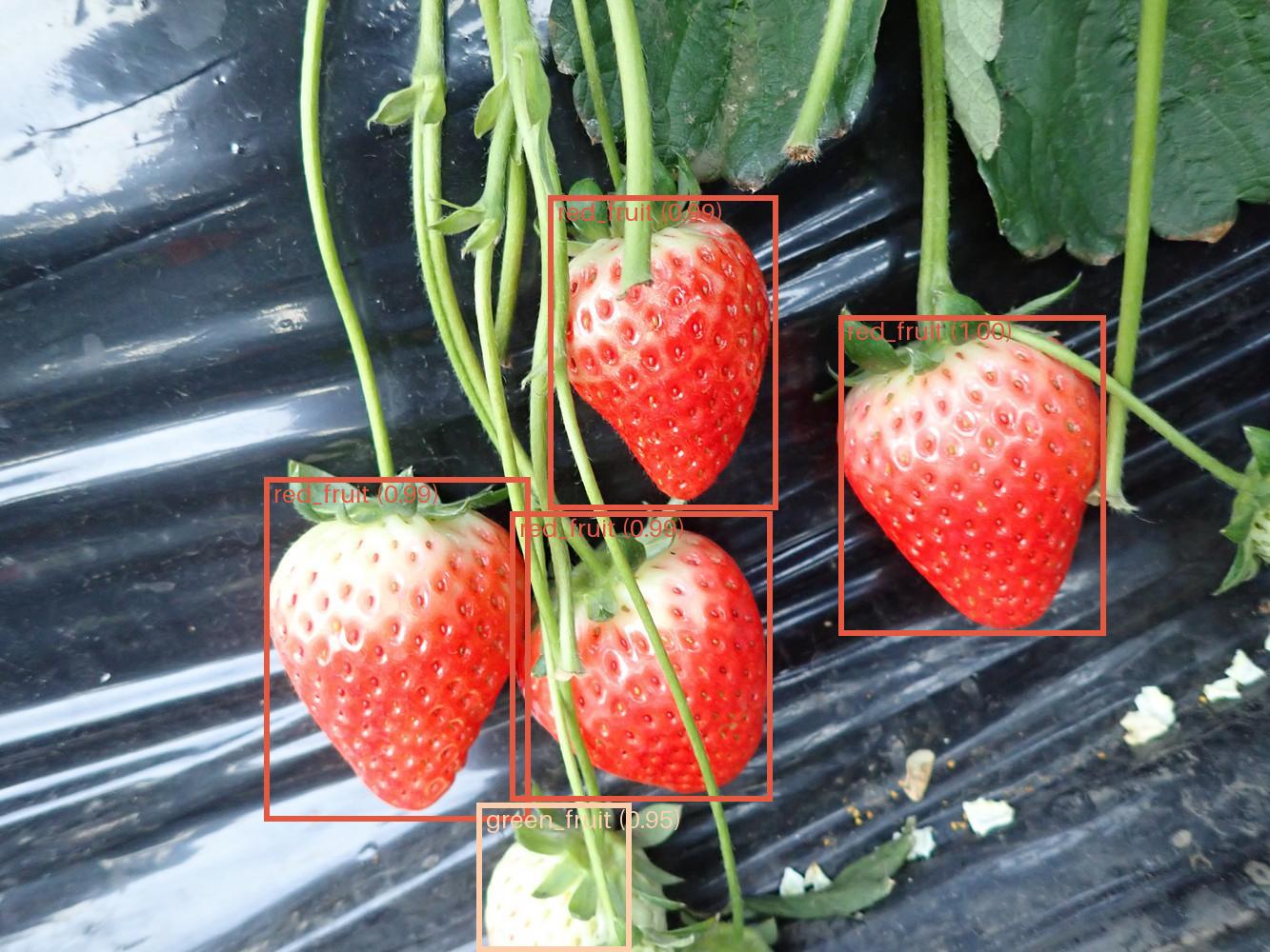
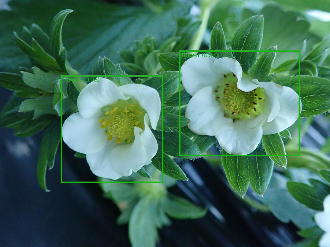
Example of outputed images are: